Multi-Mission MAG

Abstract: An introduction to “the greater Swarm”: calibrated platform magnetometer data from other missions. We begin with Cryosat-2, GRACE, GRACE-FO, and GOCE

See also:

• https://nbviewer.jupyter.org/github/pacesm/jupyter_notebooks/blob/master/MAG

SERVER_URL = "https://vires.services/ows"

%load_ext watermark
%watermark -i -v -p viresclient,pandas,xarray,matplotlib,cartopy

Python implementation: CPython
Python version       : 3.11.6
IPython version      : 8.18.0

viresclient: 0.11.6
pandas     : 2.1.3
xarray     : 2023.12.0
matplotlib : 3.8.2
cartopy    : 0.22.0

from viresclient import SwarmRequest
import datetime as dt
import matplotlib.pyplot as plt
import cartopy.crs as ccrs
import cartopy.feature as cfeature
from tqdm.notebook import tqdm

Product information

Platform magnetometer data from other missions have been carefully recalibrated so that they are accurate and suitable for usage in geomagnetic field modelling. The data currently available from VirES are as follows:

• CryoSat-2:
  Olsen, N., Albini, G., Bouffard, J. et al., Magnetic observations from CryoSat-2: calibration and processing of satellite platform magnetometer data. Earth Planets Space 72, 48 (2020).
  https://doi.org/10.1186/s40623-020-01171-9
  VirES collection names: "CS_OPER_MAG"

• GRACE (x2):
  Olsen, N., Magnetometer data from the GRACE satellite duo. Earth Planets Space 73, 62 (2021).
  https://doi.org/10.1186/s40623-021-01373-9
  VirES collection names: "GRACE_A_MAG", "GRACE_B_MAG"

• GRACE-FO (x2):
  Stolle, C., Michaelis, I., Xiong, C. et al., Observing Earth’s magnetic environment with the GRACE-FO mission. Earth Planets Space 73, 51 (2021).
  https://doi.org/10.1186/s40623-021-01364-w
  VirES collection names: "GF1_OPER_FGM_ACAL_CORR", "GF2_OPER_FGM_ACAL_CORR"

• GOCE:
  Michaelis, Ingo; Korte, Monika (2022), GOCE calibrated and characterised magnetometer data. V. 0205. GFZ Data Services.
  https://doi.org/10.5880/GFZ.2.3.2022.001
  VirES collection names: "GO_MAG_ACAL_CORR"

• GOCE (ML-calibrated):
  Styp-Rekowski, Kevin; Michaelis, Ingo; Stolle, Claudia; Baerenzung, Julien; Korte, Monika; Kao, Odej (2022): GOCE ML-calibrated magnetic field data. V. 0204. GFZ Data Services.
  https://doi.org/10.5880/GFZ.2.3.2022.002
  VirES collection names: "GO_MAG_ACAL_CORR_ML"

The variables available from each collection are:

request = SwarmRequest(SERVER_URL)
for collection in ("CS_OPER_MAG", "GRACE_A_MAG", "GF1_OPER_FGM_ACAL_CORR", "GO_MAG_ACAL_CORR"):
    print(f"{collection}:\n{request.available_measurements(collection)}\n")

CS_OPER_MAG:
['F', 'B_NEC', 'B_mod_NEC', 'B_NEC1', 'B_NEC2', 'B_NEC3', 'B_FGM1', 'B_FGM2', 'B_FGM3', 'q_NEC_CRF', 'q_error']

GRACE_A_MAG:
['F', 'B_NEC', 'B_NEC_raw', 'B_FGM', 'q_NEC_CRF', 'q_error']

GF1_OPER_FGM_ACAL_CORR:
['F', 'B_NEC', 'B_FGM', 'dB_MTQ_FGM', 'dB_XI_FGM', 'dB_NY_FGM', 'dB_BT_FGM', 'dB_ST_FGM', 'dB_SA_FGM', 'dB_BAT_FGM', 'q_NEC_FGM', 'B_FLAG']

GO_MAG_ACAL_CORR:
['F', 'B_MAG', 'B_NEC', 'dB_MTQ_SC', 'dB_XI_SC', 'dB_NY_SC', 'dB_BT_SC', 'dB_ST_SC', 'dB_SA_SC', 'dB_BAT_SC', 'dB_HK_SC', 'dB_BLOCK_CORR', 'q_SC_NEC', 'q_MAG_SC', 'B_FLAG']

Where additional B_NEC variables are specified (B_NEC1, B_NEC2, B_NEC3), these correspond to measurements from separate magnetometers on-board the spacecraft. See the scientific publications for details. Magnetic model evaluation will also work with those variables.

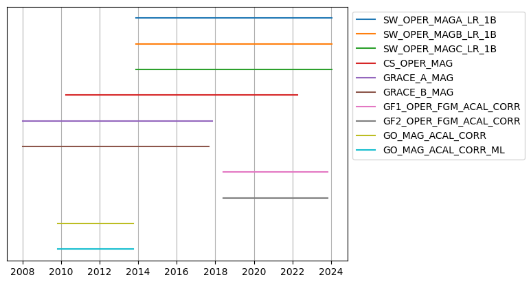
The temporal availabilities of data are:

availabilities = {}
for collection in (
    "SW_OPER_MAGA_LR_1B", "SW_OPER_MAGB_LR_1B", "SW_OPER_MAGC_LR_1B",
    "CS_OPER_MAG",
    "GRACE_A_MAG", "GRACE_B_MAG",
    "GF1_OPER_FGM_ACAL_CORR", "GF2_OPER_FGM_ACAL_CORR",
    "GO_MAG_ACAL_CORR", "GO_MAG_ACAL_CORR_ML",
):
    df = request.available_times(collection)
    start = df["starttime"].iloc[0].to_pydatetime()
    end = df["endtime"].iloc[-1].to_pydatetime()
    availabilities[collection] = (start, end)
for collection, (start, end) in availabilities.items():
    print(f"{collection}:\n {start.isoformat()} to {end.isoformat()}")

SW_OPER_MAGA_LR_1B:
 2013-11-25T11:02:52+00:00 to 2024-01-20T23:59:59.001000+00:00
SW_OPER_MAGB_LR_1B:
 2013-11-25T11:01:15+00:00 to 2024-01-20T23:59:59.001000+00:00
SW_OPER_MAGC_LR_1B:
 2013-11-25T11:02:17+00:00 to 2024-01-20T23:59:59.001000+00:00
CS_OPER_MAG:
 2010-04-08T17:03:26.254008+00:00 to 2022-03-31T23:59:52.267008+00:00
GRACE_A_MAG:
 2008-01-01T00:00:04.787680+00:00 to 2017-10-31T23:59:38.946023+00:00
GRACE_B_MAG:
 2008-01-01T00:00:04.971828+00:00 to 2017-09-04T15:11:05.000953+00:00
GF1_OPER_FGM_ACAL_CORR:
 2018-06-01T00:00:00+00:00 to 2023-10-31T23:59:59.001000+00:00
GF2_OPER_FGM_ACAL_CORR:
 2018-06-01T00:00:00+00:00 to 2023-10-31T23:59:59.001000+00:00
GO_MAG_ACAL_CORR:
 2009-11-01T00:49:15.411000+00:00 to 2013-09-30T02:47:35.587000+00:00
GO_MAG_ACAL_CORR_ML:
 2009-11-01T00:49:15.411000+00:00 to 2013-09-30T02:47:35.587000+00:00

fig, ax = plt.subplots(1, 1)
for i, (collection, (start, end)) in enumerate(availabilities.items()):
    ax.plot([start, end], [-i, -i], label=collection)
ax.legend(bbox_to_anchor=(1, 1, 0, 0))
ax.set_yticks([])
ax.grid()

Access works just like Swarm MAG products

We can specify which collection to fetch, and which models to evaluate at the same time:

request = SwarmRequest()
request.set_collection("GF1_OPER_FGM_ACAL_CORR")
request.set_products(["B_NEC"], models=["IGRF"])
data = request.get_between("2018-06-01", "2018-06-02")
ds = data.as_xarray()
ds

<xarray.Dataset>
Dimensions:     (Timestamp: 86400, NEC: 3)
Coordinates:
  * Timestamp   (Timestamp) datetime64[ns] 2018-06-01 ... 2018-06-01T23:59:59
  * NEC         (NEC) <U1 'N' 'E' 'C'
Data variables:
    Spacecraft  (Timestamp) object '1' '1' '1' '1' '1' ... '1' '1' '1' '1' '1'
    Latitude    (Timestamp) float64 15.74 15.8 15.86 15.93 ... 83.02 82.95 82.89
    Longitude   (Timestamp) float64 -11.27 -11.27 -11.27 ... 159.1 159.2 159.3
    Radius      (Timestamp) float64 6.881e+06 6.881e+06 ... 6.873e+06 6.873e+06
    B_NEC       (Timestamp, NEC) float64 2.527e+04 -2.319e+03 ... 4.648e+04
    B_NEC_IGRF  (Timestamp, NEC) float64 2.528e+04 -2.316e+03 ... 4.647e+04
Attributes:
    Sources:         ['GF1_OPER_FGM_ACAL_CORR_20180601T000000_20180601T235959...
    MagneticModels:  ['IGRF = IGRF(max_degree=13,min_degree=1)']
    AppliedFilters:  []

xarray.Dataset

• Dimensions:
  • Timestamp: 86400
  • NEC: 3
• Coordinates: (2)
  • Timestamp
    (Timestamp)
    datetime64[ns]
    2018-06-01 ... 2018-06-01T23:59:59

    description :

    Timestamp

    array(['2018-06-01T00:00:00.000000000', '2018-06-01T00:00:01.000000000',
           '2018-06-01T00:00:02.000000000', ..., '2018-06-01T23:59:57.000000000',
           '2018-06-01T23:59:58.000000000', '2018-06-01T23:59:59.000000000'],
          dtype='datetime64[ns]')

  • NEC
    (NEC)
    <U1
    'N' 'E' 'C'

    units :

    description :

    NEC frame - North, East, Centre (down)

    array(['N', 'E', 'C'], dtype='<U1')

• Data variables: (6)
  • Spacecraft
    (Timestamp)
    object
    '1' '1' '1' '1' ... '1' '1' '1' '1'

    units :

    -

    description :

    Spacecraft identifier (values: 'A', 'B', 'C' or '-' if not available).

    array(['1', '1', '1', ..., '1', '1', '1'], dtype=object)

  • Latitude
    (Timestamp)
    float64
    15.74 15.8 15.86 ... 82.95 82.89

    units :

    description :

    array([15.73672507, 15.80007206, 15.86341902, ..., 83.01550957,
           82.95274033, 82.88995937])

  • Longitude
    (Timestamp)
    float64
    -11.27 -11.27 ... 159.2 159.3

    units :

    description :

    array([-11.26783387, -11.27081412, -11.27379361, ..., 159.11290222,
           159.18325716, 159.2523027 ])

  • Radius
    (Timestamp)
    float64
    6.881e+06 6.881e+06 ... 6.873e+06

    units :

    description :

    array([6881136.2505792 , 6881134.23684505, 6881132.20983972, ...,
           6873032.62493092, 6873026.74420539, 6873020.87086135])

  • B_NEC
    (Timestamp, NEC)
    float64
    2.527e+04 -2.319e+03 ... 4.648e+04

    units :

    nT

    description :

    [nT] Fluxgate magnetometer, FGM, aligned, vector-vector calibrated and corrected for satellite disturbances, NEC frame

    array([[25270.7807418 , -2319.44292664,  5277.77857109],
           [25274.30848294, -2316.88338998,  5346.61520589],
           [25277.51296352, -2312.45674281,  5414.97947303],
           ...,
           [ 1846.6739696 ,    96.14831229, 46469.2155814 ],
           [ 1870.54132636,    95.05255991, 46472.27676413],
           [ 1896.00231802,    99.95510353, 46476.24025829]])

  • B_NEC_IGRF
    (Timestamp, NEC)
    float64
    2.528e+04 -2.316e+03 ... 4.647e+04

    units :

    nT

    description :

    Magnetic field vector, NEC frame, calculated by the IGRF spherical harmonic model

    array([[ 2.52769144e+04, -2.31617147e+03,  5.27224414e+03],
           [ 2.52811113e+04, -2.31237375e+03,  5.34126605e+03],
           [ 2.52851912e+04, -2.30858139e+03,  5.41029983e+03],
           ...,
           [ 2.00412599e+03,  3.65105335e+01,  4.64640340e+04],
           [ 2.03340781e+03,  3.17231117e+01,  4.64660175e+04],
           [ 2.06274081e+03,  2.69645176e+01,  4.64679356e+04]])

• Indexes: (2)
  • Timestamp
    PandasIndex

    PandasIndex(DatetimeIndex(['2018-06-01 00:00:00', '2018-06-01 00:00:01',
                   '2018-06-01 00:00:02', '2018-06-01 00:00:03',
                   '2018-06-01 00:00:04', '2018-06-01 00:00:05',
                   '2018-06-01 00:00:06', '2018-06-01 00:00:07',
                   '2018-06-01 00:00:08', '2018-06-01 00:00:09',
                   ...
                   '2018-06-01 23:59:50', '2018-06-01 23:59:51',
                   '2018-06-01 23:59:52', '2018-06-01 23:59:53',
                   '2018-06-01 23:59:54', '2018-06-01 23:59:55',
                   '2018-06-01 23:59:56', '2018-06-01 23:59:57',
                   '2018-06-01 23:59:58', '2018-06-01 23:59:59'],
                  dtype='datetime64[ns]', name='Timestamp', length=86400, freq=None))

  • NEC
    PandasIndex

    PandasIndex(Index(['N', 'E', 'C'], dtype='object', name='NEC'))

• Attributes: (3)

  Sources :

  ['GF1_OPER_FGM_ACAL_CORR_20180601T000000_20180601T235959_0201', 'SW_OPER_AUX_IGR_2__19000101T000000_20241231T235959_0103']

  MagneticModels :

  ['IGRF = IGRF(max_degree=13,min_degree=1)']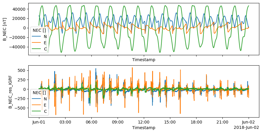

  AppliedFilters :

  []

# Append the residual, B - IGRF
ds["B_NEC_res_IGRF"] = ds["B_NEC"] - ds["B_NEC_IGRF"]
# Plot (B) and (B - IGRF) to compare
fig, axes = plt.subplots(nrows=2, ncols=1, figsize=(10, 5), sharex=True)
ds["B_NEC"].plot.line(x="Timestamp", ax=axes[0])
ds["B_NEC_res_IGRF"].plot.line(x="Timestamp", ax=axes[1]);

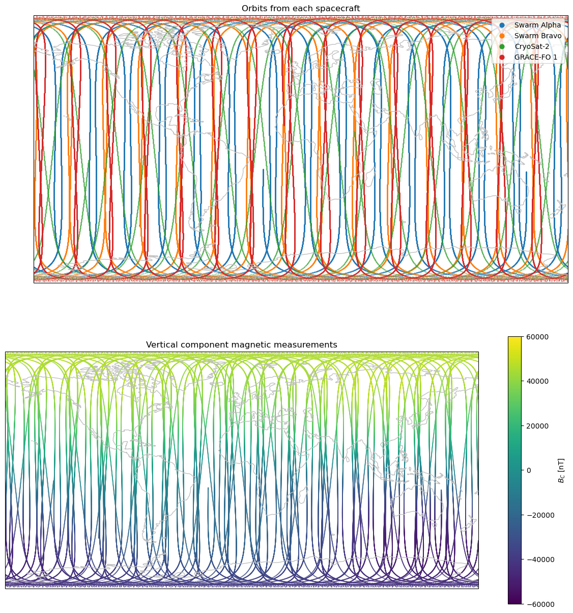
Data from multiple spacecraft

Here is an example of fetching and visualising data from multiple spacecraft. We select a day where we can get data from Swarm, CryoSat, and GRACE-FO.

START = dt.datetime(2018, 6, 1)
END = dt.datetime(2018, 6, 2)

# Mappings to identify spacecraft and collection names
# Let's disable Swarm Charlie & GRACE-FO 2 for now
#   as they are in similar places as Swarm Alpha and GRACE-FO 1
spacecraft_to_collections = {
    "Swarm Alpha": "SW_OPER_MAGA_LR_1B",
    "Swarm Bravo": "SW_OPER_MAGB_LR_1B",
    # "Swarm Charlie": "SW_OPER_MAGC_LR_1B",
    "CryoSat-2": "CS_OPER_MAG",
    "GRACE-FO 1": "GF1_OPER_FGM_ACAL_CORR",
    # "GRACE-FO 2": "GF2_OPER_FGM_ACAL_CORR"
}
collections_to_spacecraft = {v: k for k, v in spacecraft_to_collections.items()}

def fetch_sc(sc_collection, start_time=START, end_time=END, **kwargs):
    """Fetch data from a specific spacecraft"""
    request = SwarmRequest(SERVER_URL)
    request.set_collection(sc_collection)
    request.set_products(["B_NEC"])
    data = request.get_between(start_time, end_time, **kwargs)
    ds = data.as_xarray()
    # Rename the Spacecraft variable to use the mission name too
    ds.Spacecraft[:] = collections_to_spacecraft[sc_collection]
    return ds

ds_set = {}
for sc in tqdm(spacecraft_to_collections.keys()):
    collection = spacecraft_to_collections[sc]
    ds_set[sc] = fetch_sc(collection, asynchronous=False, show_progress=False)

Data are now stored within datasets within a dictionary:

ds_set["Swarm Alpha"]

<xarray.Dataset>
Dimensions:     (Timestamp: 86400, NEC: 3)
Coordinates:
  * Timestamp   (Timestamp) datetime64[ns] 2018-06-01 ... 2018-06-01T23:59:59
  * NEC         (NEC) <U1 'N' 'E' 'C'
Data variables:
    Spacecraft  (Timestamp) object 'Swarm Alpha' 'Swarm Alpha' ... 'Swarm Alpha'
    Latitude    (Timestamp) float64 -13.68 -13.74 -13.81 ... -15.43 -15.37 -15.3
    Longitude   (Timestamp) float64 -25.48 -25.48 -25.48 ... 151.8 151.8 151.8
    B_NEC       (Timestamp, NEC) float64 1.488e+04 -5.48e+03 ... -2.469e+04
    Radius      (Timestamp) float64 6.82e+06 6.82e+06 ... 6.82e+06 6.82e+06
Attributes:
    Sources:         ['SW_OPER_MAGA_LR_1B_20180601T000000_20180601T235959_060...
    MagneticModels:  []
    AppliedFilters:  []

xarray.Dataset

• Dimensions:
  • Timestamp: 86400
  • NEC: 3
• Coordinates: (2)
  • Timestamp
    (Timestamp)
    datetime64[ns]
    2018-06-01 ... 2018-06-01T23:59:59

    description :

    Time stamp

    array(['2018-06-01T00:00:00.000000000', '2018-06-01T00:00:01.000000000',
           '2018-06-01T00:00:02.000000000', ..., '2018-06-01T23:59:57.000000000',
           '2018-06-01T23:59:58.000000000', '2018-06-01T23:59:59.000000000'],
          dtype='datetime64[ns]')

  • NEC
    (NEC)
    <U1
    'N' 'E' 'C'

    units :

    description :

    NEC frame - North, East, Centre (down)

    array(['N', 'E', 'C'], dtype='<U1')

• Data variables: (5)
  • Spacecraft
    (Timestamp)
    object
    'Swarm Alpha' ... 'Swarm Alpha'

    units :

    -

    description :

    Spacecraft identifier (values: 'A', 'B', 'C' or '-' if not available).

    array(['Swarm Alpha', 'Swarm Alpha', 'Swarm Alpha', ..., 'Swarm Alpha',
           'Swarm Alpha', 'Swarm Alpha'], dtype=object)

  • Latitude
    (Timestamp)
    float64
    -13.68 -13.74 ... -15.37 -15.3

    units :

    deg

    description :

    Position in ITRF - Latitude

    array([-13.6807024, -13.7448496, -13.8089966, ..., -15.4304867,
           -15.3663387, -15.3021904])

  • Longitude
    (Timestamp)
    float64
    -25.48 -25.48 ... 151.8 151.8

    units :

    deg

    description :

    Position in ITRF - Longitude

    array([-25.4806632, -25.4816987, -25.4827325, ..., 151.8023023,
           151.8013164, 151.8003286])

  • B_NEC
    (Timestamp, NEC)
    float64
    1.488e+04 -5.48e+03 ... -2.469e+04

    units :

    nT

    description :

    Magnetic field vector, NEC frame

    array([[ 14878.0336,  -5480.1902, -14287.8419],
           [ 14854.0707,  -5478.099 , -14305.7849],
           [ 14830.1416,  -5475.9759, -14323.6677],
           ...,
           [ 26954.239 ,   3668.6557, -24821.3056],
           [ 26972.6676,   3665.8231, -24753.6346],
           [ 26990.9294,   3663.1639, -24686.073 ]])

  • Radius
    (Timestamp)
    float64
    6.82e+06 6.82e+06 ... 6.82e+06

    units :

    m

    description :

    Position in ITRF - Radius

    array([6820439.11, 6820447.98, 6820456.85, ..., 6820302.14, 6820293.43,
           6820284.71])

• Indexes: (2)
  • Timestamp
    PandasIndex

    PandasIndex(DatetimeIndex(['2018-06-01 00:00:00', '2018-06-01 00:00:01',
                   '2018-06-01 00:00:02', '2018-06-01 00:00:03',
                   '2018-06-01 00:00:04', '2018-06-01 00:00:05',
                   '2018-06-01 00:00:06', '2018-06-01 00:00:07',
                   '2018-06-01 00:00:08', '2018-06-01 00:00:09',
                   ...
                   '2018-06-01 23:59:50', '2018-06-01 23:59:51',
                   '2018-06-01 23:59:52', '2018-06-01 23:59:53',
                   '2018-06-01 23:59:54', '2018-06-01 23:59:55',
                   '2018-06-01 23:59:56', '2018-06-01 23:59:57',
                   '2018-06-01 23:59:58', '2018-06-01 23:59:59'],
                  dtype='datetime64[ns]', name='Timestamp', length=86400, freq=None))

  • NEC
    PandasIndex

    PandasIndex(Index(['N', 'E', 'C'], dtype='object', name='NEC'))

• Attributes: (3)

  Sources :

  ['SW_OPER_MAGA_LR_1B_20180601T000000_20180601T235959_0602_MDR_MAG_LR']

  MagneticModels :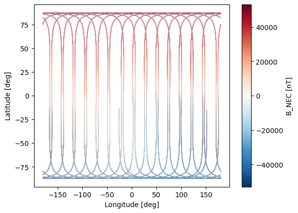

  []

  AppliedFilters :

  []

A quick inspection of the data:

ds_set["Swarm Alpha"].plot.scatter(x="Longitude", y="Latitude", hue="B_NEC", s=1, linewidths=0);

fig, axes = plt.subplots(
    nrows=2, figsize=(15,15),
    subplot_kw={"projection": ccrs.PlateCarree()}
)
for ax in axes:
    ax.add_feature(cfeature.COASTLINE, edgecolor='silver')
for sc in ("Swarm Alpha", "Swarm Bravo", "CryoSat-2", "GRACE-FO 1"):
    # Extract from dataset and plot contents
    _ds = ds_set[sc]
    lon, lat = _ds["Longitude"], _ds["Latitude"]
    B_C = _ds["B_NEC"].sel(NEC="C").values
    # Plot positions coloured by spacecraft
    axes[0].scatter(x=lon, y=lat, s=0.1, label=sc)
    # Plot vertical magnetic field
    norm = plt.Normalize(vmin=-60000, vmax=60000)
    cmap = "viridis"
    axes[1].scatter(x=lon, y=lat, c=B_C, s=0.1, norm=norm, cmap=cmap)
fig.colorbar(plt.cm.ScalarMappable(norm=norm, cmap=cmap), ax=axes[1], label=r"$B_C$ [nT]");
axes[0].legend(loc="upper right", markerscale=20)
axes[0].set_title("Orbits from each spacecraft")
axes[1].set_title("Vertical component magnetic measurements");