Swarm access through VirES

Abstract: VirES is a server/client architecture to help access time series of Swarm data and models. Access is enabled through a token generated on the website, and a Python package, viresclient, which provides the connection with the Python ecosystem (e.g. xarray).

# Display important package versions used
%load_ext watermark
%watermark -i -v -p viresclient,pandas,xarray,matplotlib

Python implementation: CPython
Python version       : 3.11.6
IPython version      : 8.18.0

viresclient: 0.11.6
pandas     : 2.1.3
xarray     : 2023.12.0
matplotlib : 3.8.2

VirES (Virtual environments for Earth Scientists) is a platform for data & model access, analysis, and visualisation for ESA’s magnetic mission, Swarm

This tutorial introduces the Python interface to VirES, viresclient. We demonstrate usage of the primary Swarm magnetic dataset (SW_OPER_MAGA_LR_1B) and geomagnetic field models produced as part of the Swarm mission. Some knowledge of pandas and matplotlib is assumed.

Run this on the VRE (Virtual Research Environment), where viresclient is already installed, or check the instructions to set it up on your own Python environment.

For more information see:

• https://vires.services/ (Web interface)

• https://viresclient.readthedocs.io (Python interface)

• https://notebooks.vires.services (Guide to Virtual Research Environment / JupyterLab)

• https://earth.esa.int/eogateway/missions/swarm (Swarm mission)

Configuration

In order to authenticate access to the VirES server, viresclient requires an access token - this ties communications between the server and the client to your account. If you are using the VRE, this is handled automatically so you can skip this step.

If you are running viresclient on a different machine, you will need to follow these instructions:

1. Create a user account at https://vires.services if you haven’t already done so

2. Install viresclient in your Python environment - see https://viresclient.readthedocs.io/en/latest/installation.html

3. Create a new code cell here and execute the following:

   from viresclient import set_token
   set_token("https://vires.services/ows", set_default=True)
   

4. You will now be directed to the VirES token management page, and prompted to generate a new token and enter it here

Your access token should now have been saved to your environment and you won’t need to provide it again. The token and its associated access URL are stored in a file: ~/.viresclient.ini (this file can also be edited directly). You may generate and set a new token, or revoke old tokens, at any point. These are similar to passwords, so should be kept secret - if you accidentally leak a token, you can revoke it at the token management page and generate a new one. It is also possible to set access tokens via CLI. For more information, see https://viresclient.readthedocs.io/en/latest/config_details.html

To remove the configuration (assuming you left it in its default location), you can use the CLI command: viresclient clear_credentials

Fetching some data

Import the SwarmRequest object which provides the VirES interface, and datetime which gives convenient time objects which can be used by SwarmRequest.get_between()

from viresclient import SwarmRequest
import datetime as dt

The following code will fetch one day (i.e. around 15 orbits) of the scalar (F) measurements from Swarm Alpha.

Several keyword arguments can be provided to .set_products() to specify the type of data you want. The measurements available depend on the collection chosen in .set_collection(). The same set of auxiliaries are available for all collections - here we also choose to fetch the MLT - magnetic local time.

sampling_step="PT10S" downsamples the data to 10 seconds, from the MAGx_LR default of 1 second. If no sampling_step is provided, the data will be accessed in its original form (i.e. here, 1-second sampling). These strings to choose the sampling_step should be provided as ISO 8601 durations (e.g. "PT1M" for 1-minute sampling).

start_time and end_time in .get_between() together provide the time window you want to fetch data for - executing this line causes the request to be processed on the server and the data returned to you. NB: this returns data up to but not including end_time. Alternatively we can provide the start and end times as ISO_8601 strings.

# Set up connection with server
request = SwarmRequest()
# Set collection to use
request.set_collection("SW_OPER_MAGA_LR_1B")
# Set mix of products to fetch:
#   measurements (variables from the given collection)
#   models (magnetic model predictions at spacecraft sampling points)
#   auxiliaries (variables available with any collection)
# Reference: https://viresclient.readthedocs.io/en/latest/available_parameters.html
# Also set additional configuration such as:
#   sampling_step
request.set_products(
    measurements=["F"],
    sampling_step="PT10S",
    auxiliaries=["MLT"]
)
# Fetch data from a given time interval
data = request.get_between(
    start_time=dt.datetime(2016,1,1),
    end_time=dt.datetime(2016,1,2)
)

The data is now contained within the object which we called data:

data

<viresclient._data_handling.ReturnedData at 0x7fac80a0cad0>

The data is temporarily stored on disk and not yet loaded into memory - the ReturnedData object is actually a wrapper around a temporary CDF file which could be written to disk directly:

# data.to_file("test_file.cdf", overwrite=True)

… but it is possible to directly transfer it to a pandas.DataFrame object:

df = data.as_dataframe()
print(type(df))
df.head()

<class 'pandas.core.frame.DataFrame'>

	Latitude	Longitude	MLT	Radius	F	Spacecraft
Timestamp
2016-01-01 00:00:00	-72.499224	92.793965	1.724749	6833853.12	46935.6044	A
2016-01-01 00:00:10	-73.130684	93.091636	1.498856	6833864.77	46908.1245	A
2016-01-01 00:00:20	-73.761536	93.414899	1.256029	6833876.01	46878.1841	A
2016-01-01 00:00:30	-74.391707	93.766830	0.996315	6833886.85	46845.8630	A
2016-01-01 00:00:40	-75.021113	94.151010	0.720387	6833897.28	46811.3661	A

… or a xarray.Dataset:

ds = data.as_xarray()
print(type(ds))
ds

<class 'xarray.core.dataset.Dataset'>

<xarray.Dataset>
Dimensions:     (Timestamp: 8640)
Coordinates:
  * Timestamp   (Timestamp) datetime64[ns] 2016-01-01 ... 2016-01-01T23:59:50
Data variables:
    Spacecraft  (Timestamp) object 'A' 'A' 'A' 'A' 'A' ... 'A' 'A' 'A' 'A' 'A'
    Latitude    (Timestamp) float64 -72.5 -73.13 -73.76 ... 29.82 30.46 31.1
    Longitude   (Timestamp) float64 92.79 93.09 93.41 ... -95.37 -95.37 -95.37
    F           (Timestamp) float64 4.694e+04 4.691e+04 ... 3.83e+04 3.861e+04
    MLT         (Timestamp) float64 1.725 1.499 1.256 ... 17.15 17.15 17.15
    Radius      (Timestamp) float64 6.834e+06 6.834e+06 ... 6.823e+06 6.823e+06
Attributes:
    Sources:         ['SW_OPER_MAGA_LR_1B_20160101T000000_20160101T235959_060...
    MagneticModels:  []
    AppliedFilters:  []

xarray.Dataset

• Dimensions:
  • Timestamp: 8640
• Coordinates: (1)
  • Timestamp
    (Timestamp)
    datetime64[ns]
    2016-01-01 ... 2016-01-01T23:59:50

    description :

    Time stamp

    array(['2016-01-01T00:00:00.000000000', '2016-01-01T00:00:10.000000000',
           '2016-01-01T00:00:20.000000000', ..., '2016-01-01T23:59:30.000000000',
           '2016-01-01T23:59:40.000000000', '2016-01-01T23:59:50.000000000'],
          dtype='datetime64[ns]')

• Data variables: (6)
  • Spacecraft
    (Timestamp)
    object
    'A' 'A' 'A' 'A' ... 'A' 'A' 'A' 'A'

    units :

    -

    description :

    Spacecraft identifier (values: 'A', 'B', 'C' or '-' if not available).

    array(['A', 'A', 'A', ..., 'A', 'A', 'A'], dtype=object)

  • Latitude
    (Timestamp)
    float64
    -72.5 -73.13 -73.76 ... 30.46 31.1

    units :

    deg

    description :

    Position in ITRF - Latitude

    array([-72.4992237, -73.1306842, -73.7615363, ...,  29.8151525,
            30.4562179,  31.0972848])

  • Longitude
    (Timestamp)
    float64
    92.79 93.09 93.41 ... -95.37 -95.37

    units :

    deg

    description :

    Position in ITRF - Longitude

    array([ 92.7939645,  93.0916362,  93.4148993, ..., -95.3651702,
           -95.3672226, -95.3687473])

  • F
    (Timestamp)
    float64
    4.694e+04 4.691e+04 ... 3.861e+04

    units :

    nT

    description :

    Magnetic field intensity

    array([46935.6044, 46908.1245, 46878.1841, ..., 37993.7923, 38304.8112,
           38613.8844])

  • MLT
    (Timestamp)
    float64
    1.725 1.499 1.256 ... 17.15 17.15

    units :

    h

    description :

    Magnetic local time

    array([ 1.72474861,  1.49885559,  1.25602913, ..., 17.1523819 ,
           17.15350723, 17.15466309])

  • Radius
    (Timestamp)
    float64
    6.834e+06 6.834e+06 ... 6.823e+06

    units :

    m

    description :

    Position in ITRF - Radius

    array([6833853.12, 6833864.77, 6833876.01, ..., 6823168.59, 6823048.61,
           6822928.78])

• Indexes: (1)
  • Timestamp
    PandasIndex

    PandasIndex(DatetimeIndex(['2016-01-01 00:00:00', '2016-01-01 00:00:10',
                   '2016-01-01 00:00:20', '2016-01-01 00:00:30',
                   '2016-01-01 00:00:40', '2016-01-01 00:00:50',
                   '2016-01-01 00:01:00', '2016-01-01 00:01:10',
                   '2016-01-01 00:01:20', '2016-01-01 00:01:30',
                   ...
                   '2016-01-01 23:58:20', '2016-01-01 23:58:30',
                   '2016-01-01 23:58:40', '2016-01-01 23:58:50',
                   '2016-01-01 23:59:00', '2016-01-01 23:59:10',
                   '2016-01-01 23:59:20', '2016-01-01 23:59:30',
                   '2016-01-01 23:59:40', '2016-01-01 23:59:50'],
                  dtype='datetime64[ns]', name='Timestamp', length=8640, freq=None))

• Attributes: (3)

  Sources :

  ['SW_OPER_MAGA_LR_1B_20160101T000000_20160101T235959_0602_MDR_MAG_LR']

  MagneticModels :

  []

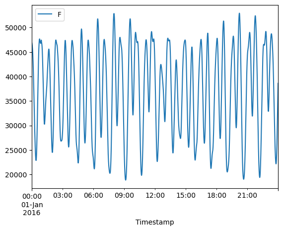
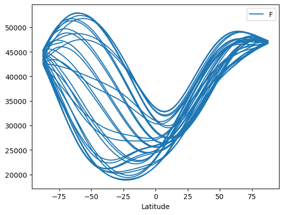
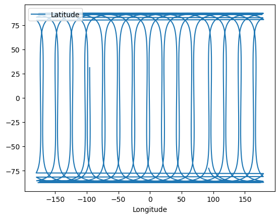
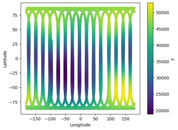
  AppliedFilters :

  []

Try plotting some things to visualise the data. The following shows the variation in field strength measured by the satellite as it passes between high and low latitudes, varying from one orbit to the next as it samples a different longitude.

df.plot(y="F")
df.plot(y="F", x="Latitude")
df.plot(y="Latitude", x="Longitude")
df.plot(y="Latitude", x="Longitude", c="F", kind="scatter");

Fetching model evaluations at the same time

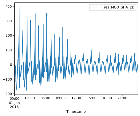
Various (spherical harmonic) models of the geomagnetic field are produced as Swarm mission products and these are available through VirES. They are evaluated on demand at the same points and times as the data sample points. Here we ask for the MCO_SHA_2D model, a dedicated core field model produced from Swarm data. By supplying residuals=True we will get the data-model residuals, named in the dataframe as F_res_MCO_SHA_2D.

request = SwarmRequest()
request.set_collection("SW_OPER_MAGA_LR_1B")
request.set_products(
    measurements=["F"],
    models=["MCO_SHA_2D"],
    residuals=True,
    sampling_step="PT10S"
)

data = request.get_between(
    start_time=dt.datetime(2016,1,1),
    end_time=dt.datetime(2016,1,2)
)

df = data.as_dataframe()
df.head()

	Latitude	Longitude	Radius	Spacecraft	F_res_MCO_SHA_2D
Timestamp
2016-01-01 00:00:00	-72.499224	92.793965	6833853.12	A	111.777750
2016-01-01 00:00:10	-73.130684	93.091636	6833864.77	A	108.079555
2016-01-01 00:00:20	-73.761536	93.414899	6833876.01	A	104.163471
2016-01-01 00:00:30	-74.391707	93.766830	6833886.85	A	100.104800
2016-01-01 00:00:40	-75.021113	94.151010	6833897.28	A	96.106717

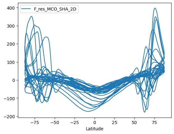
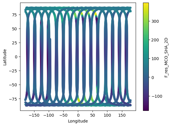
The core field has been removed from the data so the amplitudes are much smaller. Can you interpret the new signals in terms of external fields, i.e. from the ionosphere and magnetosphere?

df.plot(y="F_res_MCO_SHA_2D")
df.plot(y="F_res_MCO_SHA_2D", x="Latitude")
df.plot(y="Latitude", x="Longitude", c="F_res_MCO_SHA_2D", kind="scatter");

More complex model handling

We can also remove a magnetospheric field model at the same time, by specifying a new model (which we call MCO_MMA here, but can be named whatever you like) which is the sum of core and magnetospheric models.

See Swarm_notebooks/notebooks/02b__viresclient-Available-Data for more examples of this - it is also possible to specify the spherical harmonic degrees (min/max) to use, and to provide your own .shc model.

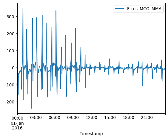
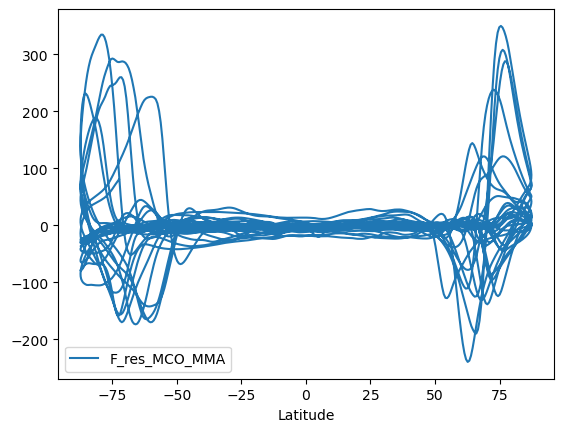
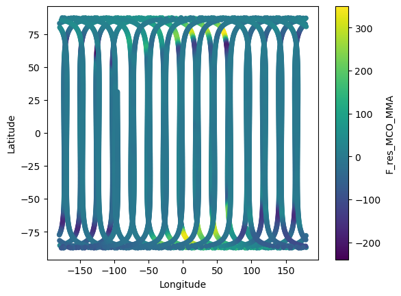
The remaining signal is now primarily due to the ionosphere.

Note that here we are instead using the CI (comprehensive inversion) core and magnetosphere models (indicated by 2C in the product names). The magnetospheric model (MMA) is split into two parts - “primary”: external to the Earth, and “secondary”: the induced counterpart internal to the Earth.

request = SwarmRequest()
request.set_collection("SW_OPER_MAGA_LR_1B")
request.set_products(
    measurements=["F"],
    models=["MCO_MMA = 'MCO_SHA_2C' + 'MMA_SHA_2C-Primary' + 'MMA_SHA_2C-Secondary'"],
    residuals=True,
    sampling_step="PT10S",
    auxiliaries=["MLT"]
)

data = request.get_between(
    start_time=dt.datetime(2016,1,1),
    end_time=dt.datetime(2016,1,2)
)

df = data.as_dataframe()
df.head()

	Latitude	F_res_MCO_MMA	Longitude	MLT	Radius	Spacecraft
Timestamp
2016-01-01 00:00:00	-72.499224	80.085681	92.793965	1.724749	6833853.12	A
2016-01-01 00:00:10	-73.130684	76.191297	93.091636	1.498856	6833864.77	A
2016-01-01 00:00:20	-73.761536	72.078270	93.414899	1.256029	6833876.01	A
2016-01-01 00:00:30	-74.391707	67.811187	93.766830	0.996315	6833886.85	A
2016-01-01 00:00:40	-75.021113	63.582477	94.151010	0.720387	6833897.28	A

df.plot(y="F_res_MCO_MMA")
df.plot(y="F_res_MCO_MMA", x="Latitude")
df.plot(y="Latitude", x="Longitude", c="F_res_MCO_MMA", kind="scatter");